Accessing, Loading, and Plotting Spatial Data in R

Analysis of Spatiotemporal Data - Session 1

Poshan Niraula

2026-11-06

Introduce yourself

Name, Country
Bachelor’s degree
Experience with programming (R/python)
Experience with data analysis (geographic data)

Today’s Goals

Installations
Refresh R fundamentals for spatial data
Understand spatial objects in R
Load, transform, and visualize spatial data
Preview spatiotemporal data structures

Why R for Spatial Data?

Advantages

Open source & reproducible
Rich spatial ecosystem
Statistical powerhouse
Growing community

Key Packages

sf - simple features
terra - raster data
stars - spatiotemporal arrays
tidyverse - data wrangling

Book reference: r-spatial.org/book - Chapters 1-3, 5-8

Part 1: R Fundamentals

R is a REPL

Read - Evaluate - Print - Loop

# Assignment: don't print
a = 3

# No assignment: print
a

[1] 3

# Interactive exploration
sqrt(a)

[1] 1.732051

Pipes: Readable Code

Traditional nesting:

sin(sqrt(sum(3:7)))

[1] -0.9589243

Modern pipes:

3:7 |> 
  sum() |>
  sqrt() |>
  sin()

[1] -0.9589243

Read as: “Take 3:7, then sum, then sqrt, then sin”

R Objects: Everything is an Object

Not only the language objects or functions, but basic “things” such as data objects.

Homogeneous vectors

# Vectors
a = c(1, 2, 3)
typeof(a)

[1] "double"

Data structure

Vector
List
Matrix
Dataframe

Indexing vectors

Access elements using [ for ranges or [[ for single elements:

# Vectors: indexing

v <- c(10, 20, 30, 40, 50)

# Single element with [[
v[[2]]

[1] 20

# Range with [
v[2:4]

[1] 20 30 40

# Multiple indices with [
v[c(1, 3, 5)]

[1] 10 30 50

Heterogenous vectors: list

# lists
l = list(name = "John", age = 25, scores = c(85, 90, 88))
l$name

[1] "John"

[ and [[ have further distinction in list
- [ returns list
- [[ returns the contents of the list element

# listretrieval
l <- list(3, TRUE, "foo")
l[1]

[[1]]
[1] 3

l[[1]]

[1] 3

Matrices

n*n array

a = 1:10
m = matrix(a, ncol = 2)
m

a = 1:10
m = matrix(a, nrow = 2)
m

     [,1] [,2] [,3] [,4] [,5]
[1,]    1    3    5    7    9
[2,]    2    4    6    8   10

R fills the columns first

Matrices

Using rbind (bindig by rows)/cbind (binding by columns)

m = rbind(1:3, 4:6)
m

     [,1] [,2] [,3]
[1,]    1    2    3
[2,]    4    5    6

m = cbind(1:3, 4:6)
m

     [,1] [,2]
[1,]    1    4
[2,]    2    5
[3,]    3    6

Data Frames

Most common data structure - like a spreadsheet!

Key Properties:

Columns can be different types
Each column = equal length
Think: Excel table
Actually a special list!

# Create a data frame
df = data.frame(
  name = c("Alice", "Bob", "Carol"),
  age = c(25, 30, 28),
  score = c(85.5, 92.0, 88.3)
)
df

   name age score
1 Alice  25  85.5
2   Bob  30  92.0
3 Carol  28  88.3

Data Frame Structure

# Check the structure
str(df)

'data.frame':   3 obs. of  3 variables:
 $ name : chr  "Alice" "Bob" "Carol"
 $ age  : num  25 30 28
 $ score: num  85.5 92 88.3

# Data frame is a list!
class(df)

[1] "data.frame"

is.list(df)

[1] TRUE

Each column is a vector in a list

Accessing Data Frame Elements

# Access column by name (returns vector)
df$name

[1] "Alice" "Bob"   "Carol"

# Access column with [[
df[["age"]]

[1] 25 30 28

# Access multiple columns with [ (returns data frame)
df[c("name", "score")]

   name score
1 Alice  85.5
2   Bob  92.0
3 Carol  88.3

Indexing Data Frames

Two dimensions: [rows, columns]

# First row, all columns
df[1, ]

   name age score
1 Alice  25  85.5

# All rows, second column
df[, 2]

[1] 25 30 28

# Specific cell: row 2, column 3
df[2, 3]

[1] 92

# Multiple rows and columns
df[1:2, c("name", "age")]

   name age
1 Alice  25
2   Bob  30

Data Frame vs Matrix

Matrix - All elements same type - Numeric operations - Homogeneous

m = matrix(1:6, nrow = 2)
m * 2  # Works!

     [,1] [,2] [,3]
[1,]    2    6   10
[2,]    4    8   12

Data Frame - Mixed types allowed - Real-world data - Heterogeneous

df = data.frame(
  id = 1:2,
  city = c("Raleigh", "Durham")
)
df

  id    city
1  1 Raleigh
2  2  Durham

Why Data Frames Matter for Spatial Data

Spatial objects are enhanced data frames!
Regular columns: attributes (name, population, etc.)
Special column: geometry (the spatial part)
All data.frame operations work!

# Preview: this is what we'll work with
library(sf)
nc = system.file("gpkg/nc.gpkg", package = "sf") |> read_sf()
class(nc)  # It's a data.frame AND an sf object!

[1] "sf"         "tbl_df"     "tbl"        "data.frame"

Part 2: Spatial Data in R

What are Simple Features?

ISO/OGC Standard

Point, LineString, Polygon
Multi* variants
Geometry collections

In R: sf package

library(sf)

# Point
st_point(c(1, 2))

# Polygon
coords = matrix(c(0,0, 1,0, 1,1, 0,1, 0,0), 
                ncol=2, byrow=TRUE)
st_polygon(list(coords))

Book reference: Chapter 1 - Getting Started

Loading Spatial Data

library(sf)
library(tidyverse)

# Load North Carolina counties
nc = system.file("gpkg/nc.gpkg", package = "sf") |>
  read_sf()

nc

Simple feature collection with 100 features and 14 fields
Geometry type: MULTIPOLYGON
Dimension:     XY
Bounding box:  xmin: -84.32385 ymin: 33.88199 xmax: -75.45698 ymax: 36.58965
Geodetic CRS:  NAD27
# A tibble: 100 × 15
    AREA PERIMETER CNTY_ CNTY_ID NAME  FIPS  FIPSNO CRESS_ID BIR74 SID74 NWBIR74
   <dbl>     <dbl> <dbl>   <dbl> <chr> <chr>  <dbl>    <int> <dbl> <dbl>   <dbl>
 1 0.114      1.44  1825    1825 Ashe  37009  37009        5  1091     1      10
 2 0.061      1.23  1827    1827 Alle… 37005  37005        3   487     0      10
 3 0.143      1.63  1828    1828 Surry 37171  37171       86  3188     5     208
 4 0.07       2.97  1831    1831 Curr… 37053  37053       27   508     1     123
 5 0.153      2.21  1832    1832 Nort… 37131  37131       66  1421     9    1066
 6 0.097      1.67  1833    1833 Hert… 37091  37091       46  1452     7     954
 7 0.062      1.55  1834    1834 Camd… 37029  37029       15   286     0     115
 8 0.091      1.28  1835    1835 Gates 37073  37073       37   420     0     254
 9 0.118      1.42  1836    1836 Warr… 37185  37185       93   968     4     748
10 0.124      1.43  1837    1837 Stok… 37169  37169       85  1612     1     160
# ℹ 90 more rows
# ℹ 4 more variables: BIR79 <dbl>, SID79 <dbl>, NWBIR79 <dbl>,
#   geom <MULTIPOLYGON [°]>

sf Object

# It's a data.frame with geometry!
class(nc)

[1] "sf"         "tbl_df"     "tbl"        "data.frame"

# Regular columns + special geometry column
names(nc)[1:5]

[1] "AREA"      "PERIMETER" "CNTY_"     "CNTY_ID"   "NAME"

st_geometry(nc) |> head(2)

Geometry set for 2 features 
Geometry type: MULTIPOLYGON
Dimension:     XY
Bounding box:  xmin: -81.74107 ymin: 36.23436 xmax: -80.90344 ymax: 36.58965
Geodetic CRS:  NAD27

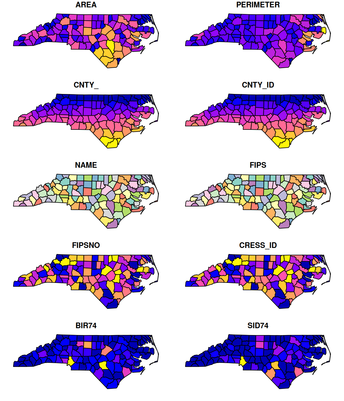
Basic Plotting

# Default plot
plot(nc)

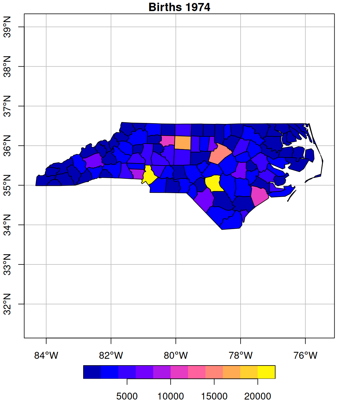
Plotting Single Variables

# Select and plot
nc |>
  select(BIR74) |>
  plot(
    main = "Births 1974",
    graticule = TRUE,
    axes = TRUE
  )

Coordinate Reference Systems

Geographic (lat/lon)

st_crs(nc)$input

[1] "NAD27"

Projected (meters)

nc_proj = nc |>
  st_transform('EPSG:32119')

st_crs(nc_proj)$input

Why CRS matters:

Distance calculations
Area calculations
Map projections
Spatial operations

Book: Chapter 2 - Coordinates

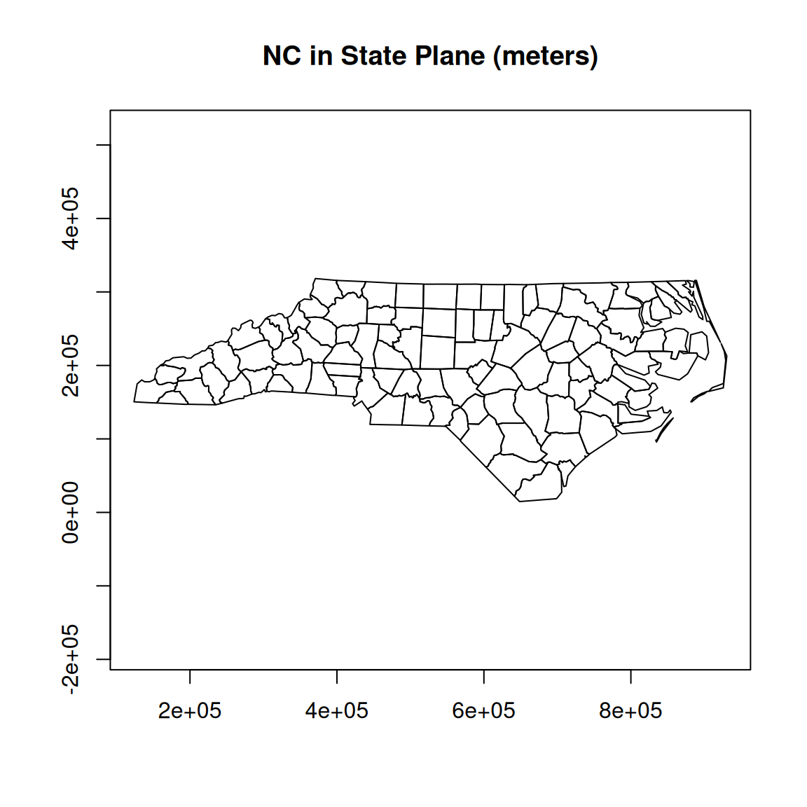
CRS Transformation

nc_proj = nc |>
  st_transform('EPSG:32119')

plot(st_geometry(nc_proj),
     main = "NC in State Plane (meters)",
     axes = TRUE)

Tidyverse + sf

Works seamlessly!

nc |>
  filter(BIR74 > 2000) |>
  select(NAME, BIR74, geom) |>
  head(3)

Simple feature collection with 3 features and 2 fields
Geometry type: MULTIPOLYGON
Dimension:     XY
Bounding box:  xmin: -80.96577 ymin: 36.16217 xmax: -78.28293 ymax: 36.56521
Geodetic CRS:  NAD27
# A tibble: 3 × 3
  NAME       BIR74                                                          geom
  <chr>      <dbl>                                            <MULTIPOLYGON [°]>
1 Surry       3188 (((-80.45634 36.24256, -80.47639 36.25473, -80.53688 36.2567…
2 Rockingham  4449 (((-79.53051 36.24614, -79.53058 36.23616, -80.02567 36.2502…
3 Vance       2180 (((-78.49252 36.17359, -78.51472 36.17522, -78.51709 36.4614…

Interactive Exercise 1

Load the nc dataset
Filter for counties where SID74 > 10
Calculate birth rate: BIR74 / BIR79
Plot the result

nc |>
  filter(SID74 > 10) |>
  mutate(birth_change = BIR74 / BIR79) |>
  select(birth_change) |>
  plot()

Part 3: Spatiotemporal Data

Spatiotemporal Data Structure

Concept: Space × Time

Spatial snapshot: Data at one time
Time series at location: One location, many times
Full spatiotemporal: Multiple locations, multiple times

Packages:

stars
spacetime

Simple Example: NC Over Time

# Add time dimension
nc_temporal = nc |>
  select(NAME, BIR74, SID74, geom) |>
  mutate(year = 1974)

nc_temporal |> head(3)

Simple feature collection with 3 features and 4 fields
Geometry type: MULTIPOLYGON
Dimension:     XY
Bounding box:  xmin: -81.74107 ymin: 36.23388 xmax: -80.43531 ymax: 36.58965
Geodetic CRS:  NAD27
# A tibble: 3 × 5
  NAME      BIR74 SID74                                               geom  year
  <chr>     <dbl> <dbl>                                 <MULTIPOLYGON [°]> <dbl>
1 Ashe       1091     1 (((-81.47276 36.23436, -81.54084 36.27251, -81.56…  1974
2 Alleghany   487     0 (((-81.23989 36.36536, -81.24069 36.37942, -81.26…  1974
3 Surry      3188     5 (((-80.45634 36.24256, -80.47639 36.25473, -80.53…  1974

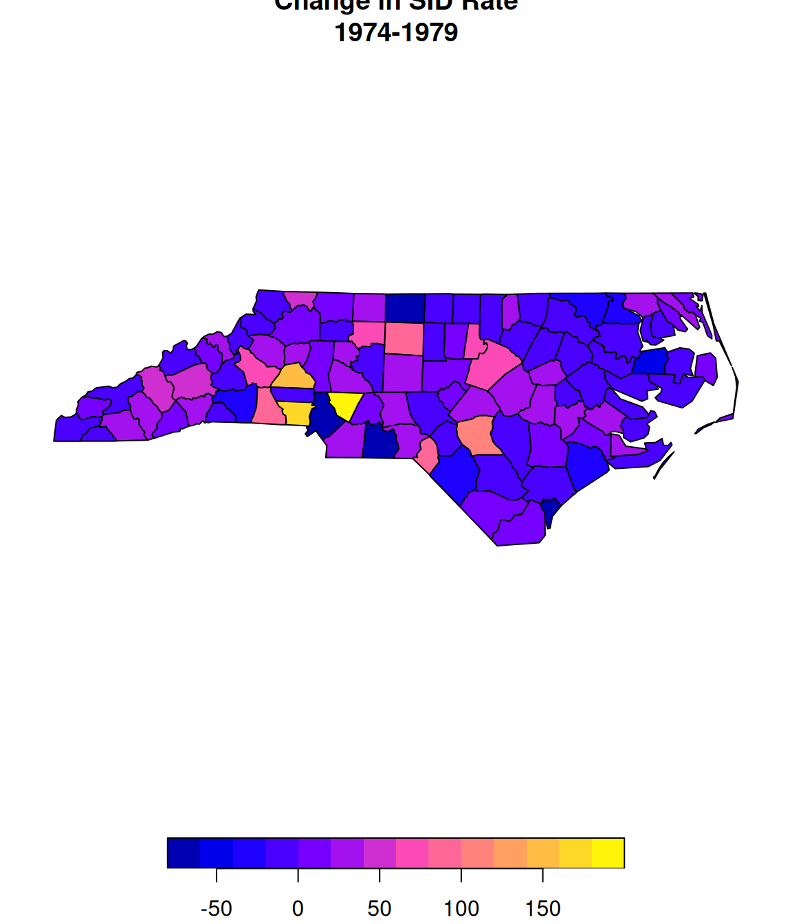
Spatial Analysis

# Simple temporal comparison
nc |>
  mutate(sid_rate_diff = 
    (SID79 - SID74) / AREA) |>
  select(sid_rate_diff) |>
  plot(main = "Change in SID Rate\n1974-1979")

Key Spatial Operations

Geometric Operations

st_buffer() - create buffers
st_intersection() - overlap
st_union() - merge
st_centroid() - centers

Predicates

st_intersects() - touches?
st_within() - inside?
st_distance() - how far?

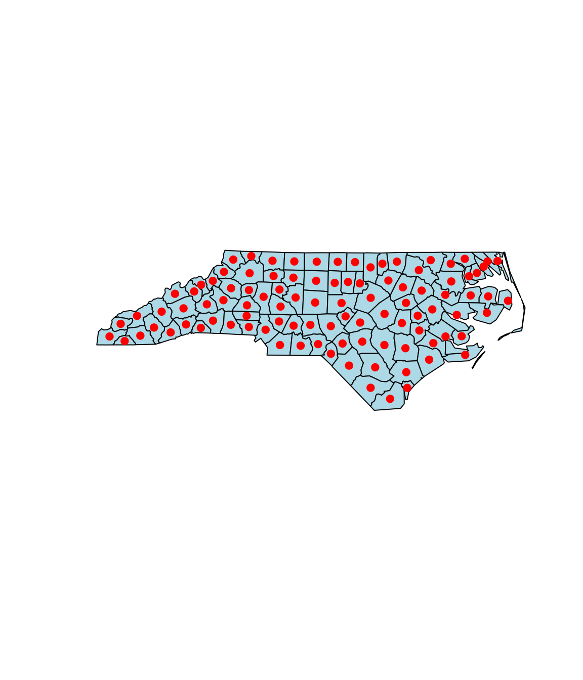
Quick Example: Centroids

nc_centers = nc |>
  st_centroid()

plot(st_geometry(nc), 
     col = "lightblue")
plot(st_geometry(nc_centers), 
     add = TRUE, 
     pch = 19, 
     col = "red")

Resources

Primary

r-spatial.org/book
sf vignettes: vignette(package="sf")

Documentation

?st_read
?st_transform
?plot.sf

Practice

Exercise session NOW!
Chapters 1-9

Quick Recap

R fundamentals: pipes, objects, workflow

Simple features: sf package, geometry types

Loading and plotting spatial data

CRS and transformations

Introduction to spatiotemporal data

Questions before exercises?

Exercise Time!

Next Hour:

Work through the Rmd exercises
Explore the nc dataset
Practice CRS transformations
Try different visualizations

Don’t hesitate to ask questions!

Other resources

Geographic data introduction https://r.geocompx.org/spatial-class

Mastering R https://r4ds.hadley.nz/