Statistical modelling of spatial data

Analysis of Spatiotemporal Data

Poshan Niraula

2026-11-06

Big picture

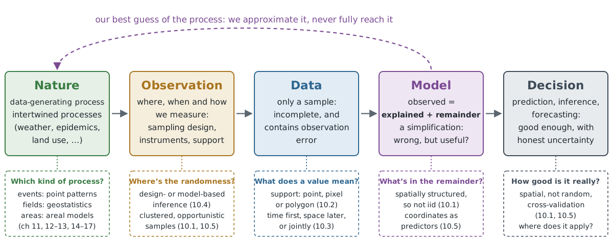
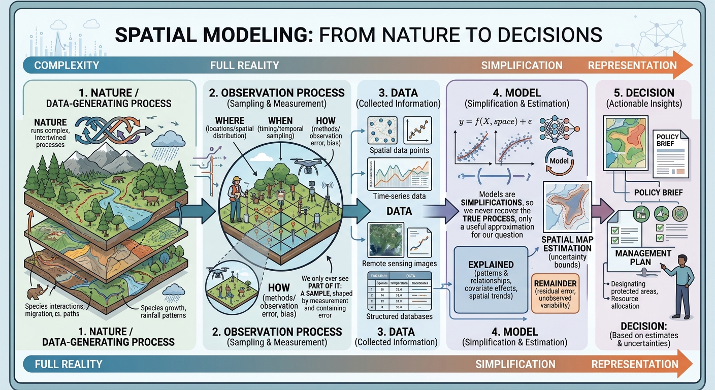
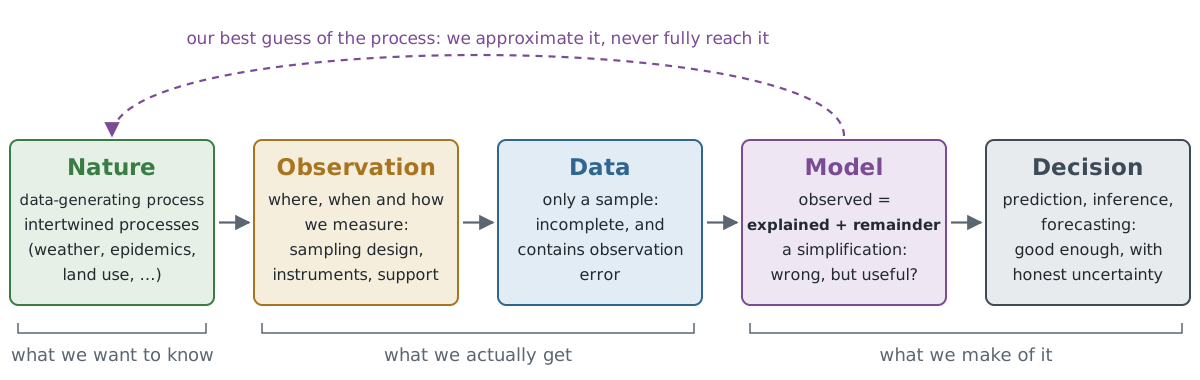
• Nature runs complex, intertwined processes; when we describe them mathematically, we call this the data-generating process.
• We only ever see part of it: a sample, shaped by where, when and how we measured, and containing observation error.
• Our models are simplifications, so we never recover the true process, only a useful approximation for our question.

Big picture

Big picture: generated using Gemini

Big picture

Big picture: generated using Claude

Analysing

• We analyse these samples to make inferences about the population,
• or to find the data-generating process, or get closer to it.
• In doing so, we:
  • quantify relationships between variables,
  • estimate population parameters, and
  • predict the outcome of observations that could have been taken but were not.

Model

• Analysis is done by adopting a model for the data, e.g.

\[\text{observed} = \text{explained} + \text{remainder}\]

• Explained: the part predicted by predictors or covariates (features in ML), e.g. with a regression model
• Remainder: the variability that could not be explained
• We may be interested in the relationship between the observed variable and the predictors, or in prediction

Example: flat rent = f(size, distance to the centre) + remainder

Model: facts

• Models will be wrong: “All models are wrong, but some are useful” (George Box)
• Choose the best of the wrong ones
• Every model has uncertainty: in predictions, relationships, etc.
• We want to be honest about these uncertainties and report them along with the results

Why the remainder matters

• The explained part gives our best guess; the remainder tells us how much to trust it
• Standard errors, p-values, confidence and prediction intervals all come from assumptions about the remainder
• Standard regression: \(y = X\beta + \varepsilon\), with \(\varepsilon\) iid \(N(0, \sigma^2)\)
• A pattern left in the remainder means the model missed something

Modelling for spatial data: the iid assumption

• iid = independent and identically distributed
  • Independent: knowing one observation tells us nothing extra about another
  • Identically distributed: all observations come from the same distribution
• Spatial data: nearby observations are similar (Tobler’s first law), and the mean often changes across space
• Temporal data: today’s temperature tells us a lot about tomorrow’s
• So we need methods that are specific to spatial and temporal data

IID or not

Which of these are (close to) iid?

• Coin flips
• Daily temperature in one city over a year
• Rents of flats in one city
• Lottery draws
• NDVI of neighbouring pixels in one field

iid: coin flips, lottery draws. Not iid: temperature (temporal), rents (spatial), NDVI (spatial).

Modelling goals for spatial and spatiotemporal data

• Predicting in space: predict a plausible value of a variable at some location, within the time span of the observations, and report the uncertainty
• Relationship finding: scientific inference about the importance of covariates
• Predicting in time: forecast the future at the same location

Modelling with non-spatial regression and ML models

• Fitting / training: with predictors and observations
• Predicting: with known predictors and unknown observations, which also gives a prediction error or interval

Modelling with non-spatial regression and ML models

library(dplyr)
library(sf)

## read file
system.file("gpkg/nc.gpkg", package = "sf") |>
    read_sf() -> nc

## create new variables
nc |> mutate(SID = SID74 / BIR74, NWB = NWBIR74 / BIR74, rate74 = SID74 / BIR74) -> nc1

lm(SID ~ NWB, nc1) |>
  predict(nc1, interval = "prediction") -> pr

bind_cols(nc, pr) |> names()

 [1] "AREA"      "PERIMETER" "CNTY_"     "CNTY_ID"   "NAME"      "FIPS"     
 [7] "FIPSNO"    "CRESS_ID"  "BIR74"     "SID74"     "NWBIR74"   "BIR79"    
[13] "SID79"     "NWBIR79"   "geom"      "fit"       "lwr"       "upr"      

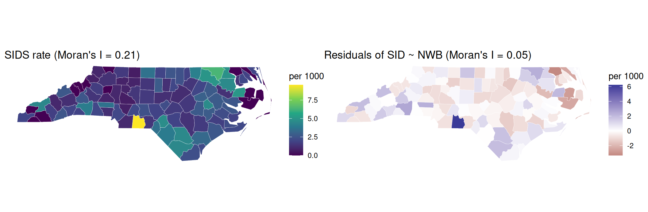
• We generally fit the model on one part of the data and predict the remaining part, to see how well the model performs.

Is there a pattern left in the remainder?

• Do neighbouring counties have similar values? Moran’s I near 0: no; larger: yes (details in ch. 14)

Model evaluation and comparison

• How do we evaluate?

Model evaluation and comparison

• Regression: RMSE, MAE, R²; classification: accuracy, kappa, ROC curve / AUC
• Cross-validation (CV) in general assumes independent observations
• Not suitable for spatial data with spatial autocorrelation and/or strong spatial clustering in the sample
• R packages that replace naive CV: spatialsample, CAST, mlr3spatial, mlr3spatiotempcv (Python: e.g. GroupKFold with spatial blocks in scikit-learn)

Support and statistical modelling

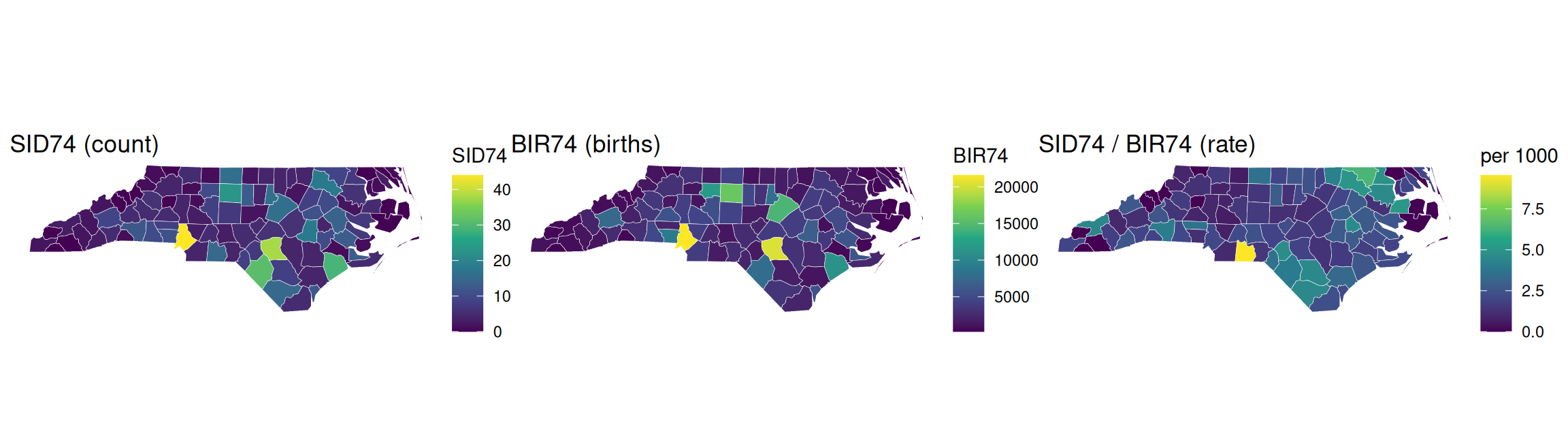
• Extensive: adds up when areas are merged, splits when they are divided (population, number of cases, births)
• Intensive: does not add up; merging gives a (weighted) average (density, rate, proportion, temperature)
• Choropleths should show intensive variables; for counts use e.g. proportional symbols

Counts, births and rates

• The count map is largely a births map: correlation between SID74 and BIR74 is 0.86

point support

Is the outcome of interest the location or the value?

Location → point patterns (ch. 11)

• Where do events happen?
• Needs all events in the observation window
• e.g. crime, trees, wildfire ignitions

Value → geostatistics (ch. 12–13)

• We choose the locations; the value measured there is the outcome
• Comes from a field that exists everywhere
• e.g. temperature, soil pH, NO₂

• Marked point patterns (tree height, earthquake magnitude): do values between the points make sense? If not, it is not geostatistics.

Summary: support

Data	Example: air quality and health	Chapters
Points: events	home locations of asthma cases	11
Points: a field	NO₂ measured at monitoring stations	12–13
Areas	asthma rates per district	14–17

• The data type follows from how the data were collected and what we ask

Time in predictive models

Ways to handle time in spatiotemporal modelling:

• Time first, space later: reduce time, then work on the problem spatially
  • e.g. hourly NO₂ at stations → annual means → interpolate a map (ch. 12)
• Space first, time later: work spatially per time step, then analyse over time
  • e.g. classify a single scene (or scenes of one season), then compare land-use / land-cover change over several years
• Jointly: model space and time together (ch. 13)

Design-based and model-based inference

Design-based

• Randomness in location is assumed
• Requires random sampling: every location has a known, positive probability of being included

Model-based

• The locations are fixed: wherever we measured
• Makes no assumption about how the samples were collected
• Inference is only valid if the assumed model is valid

Which to choose?

• Model-based framework:
  • predictions are required for individual locations, or for areas too small to be sampled
  • data were not collected with a random sampling scheme
• Design-based framework:
  • observations were collected through a random sampling process
  • aggregated properties of the entire sampled region are needed
  • estimates are required that are not sensitive to model misspecification
• If you can plan the sampling: sample randomly, it keeps both options open

Design-based: examples

• Soil carbon reporting: total carbon stock of a farm or region for a climate report or carbon credits
• Forest inventories: total timber volume or forest area of a country, from a randomly placed grid of field plots

Predictive models with coordinates

• How about adding coordinates as features / predictors?
• As with any predictor, choose methods that are not sensitive to shifts in origin or unit (scale)
  • origin: same places, different numbers (e.g. UTM false easting vs. a local grid)
  • unit: metres vs. kilometres
• Linear models with an intercept and random forests are fine; distance-based methods (kNN) and penalised regression need standardised predictors

Predictive models with coordinates: rotation

• When used as separate terms (x, y, x², y²), coordinates are sensitive to rotation of the axes (e.g. different projection systems)
• Coordinates should be used jointly, not as separate features,
  • polynomials: include the cross term, e.g. \((x + y)^2\) instead of \(x^2 + y^2\)
  • GAMs: \(s(x, y)\) instead of \(s(x) + s(y)\)
  • random forests: split along the axes; adding rotated coordinates helps

Predictive models with coordinates

• Can you think of a case where a single coordinate (lat or lon) works naturally in predictive modelling?

Latitude: yearly solar energy, day length, large-scale temperature gradients. There the north–south direction has physical meaning.

Ellipsoidal vs. projected coordinates

• Small areas: projected and ellipsoidal coordinates give similar results
• Larger areas: they differ more, and every projection distorts distances differently
• Global models with polynomials or splines in lat/lon:
  • longitude wraps around: 179.9°E and 179.9°W are neighbours, but 360 apart as numbers
  • near the poles all longitudes meet: one degree of longitude is about 111 km at the equator and almost 0 at the poles
• Use functions that are continuous on the sphere, e.g. spherical harmonics

Group discussion

• Groups of 4
• Pick one topic you find interesting; it can be an idea for your seminar project
• 10 min discussing, then 10 min sharing
• Write your answers in the shared document:

Questions for your topic

1. Question: what do you want to know? (one sentence)
2. Support: what does one value stand for: a point, a pixel or an area? Over what time?
3. Data type: events (point pattern), a field measured at points (geostatistics) or values per area (areal data)?
4. Goal: prediction (a map, a forecast) or inference (understanding a relationship)?
5. Data collection: random sampling or “whatever is available”? So design-based or model-based?

Bonus: which predictors would you use, and what could go wrong?

Need inspiration?

• Urban heat on summer nights
• Air quality (NO₂, particulate matter)
• Bicycle accidents
• Flood damage
• Deforestation

• Crop yield
• Disease cases
• House prices or rents
• Wildfires
• Species sightings

Example: urban heat

Question	Example answer
Question	Where is the city hottest on summer nights, and does green space help?
Support	Temperature at a sensor (point), or a satellite pixel (e.g. 30 m to 1 km); hourly or nightly values
Data type	A field measured at points: geostatistics (or pixels covering the whole city)
Goal	Both: a map (prediction) and the effect of green space (inference)
Data collection	Sensors placed where volunteers live: not random, so model-based
Bonus	Predictors: green space, building density, distance to water. Risk: sensors cluster in some districts, so random CV looks too good

Sharing

• Each group: your topic and your answers in one minute
• Did two groups pick similar topics but different data types or supports?
• Was anyone design-based?

Take-home messages

1. A model = what we can explain + what is left over (the remainder)
2. In spatial data, nearby values are similar, and so are their leftovers
3. Similar observations carry less information than their number suggests: standard errors and random CV become too optimistic
4. Random sampling: design-based; data from wherever we could get them: model-based
5. Always ask: what does one value stand for (point, pixel or area)?

Summary

Big picture: generated using Claude

Next steps

• Exercise: now
• Next week: point pattern analysis (ch. 11)
• Seminar project: aim and data, due before 13 Nov;

Exercise Time!

Exercise 1

 [1] "AREA"      "PERIMETER" "CNTY_"     "CNTY_ID"   "NAME"      "FIPS"     
 [7] "FIPSNO"    "CRESS_ID"  "BIR74"     "SID74"     "NWBIR74"   "BIR79"    
[13] "SID79"     "NWBIR79"   "geom"      "fit"       "lwr"       "upr"      

Exercise 3

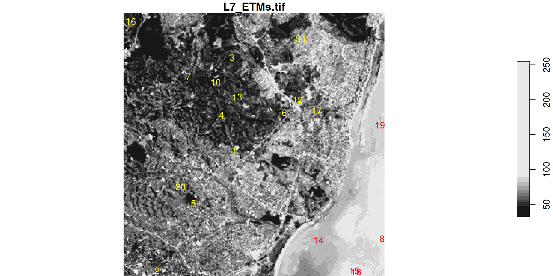
stars object with 3 dimensions and 1 attribute
attribute(s):
             Min. 1st Qu. Median     Mean 3rd Qu. Max.
L7_ETMs.tif     1      54     69 68.91242      86  255
dimension(s):
     from  to  offset delta                     refsys point x/y
x       1 349  288776  28.5 SIRGAS 2000 / UTM zone 25S FALSE [x]
y       1 352 9120761 -28.5 SIRGAS 2000 / UTM zone 25S FALSE [y]
band    1   6      NA    NA                         NA    NA    

stars object with 2 dimensions and 1 attribute
attribute(s):
             Min. 1st Qu. Median     Mean 3rd Qu. Max.
L7_ETMs.tif    12   41.75     63 60.95833    80.5  145
dimension(s):
         from to                     refsys point
geometry    1 20 SIRGAS 2000 / UTM zone 25S  TRUE
band        1  6                         NA    NA
                                                        values
geometry POINT (293002.2 9115516),...,POINT (290941.1 9114128)
band                                                      NULL

NULL

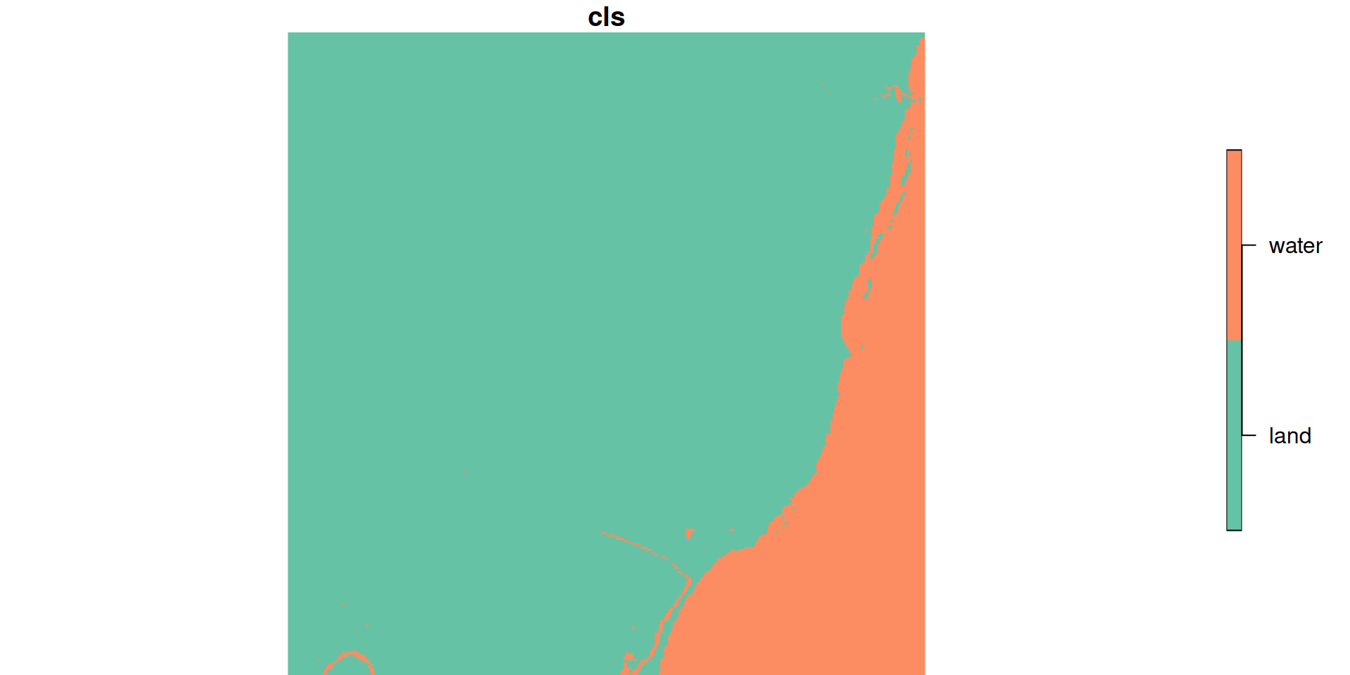
classification task