Point pattern analysis

Analysis of Spatiotemporal Data

Poshan Niraula

2026-11-06

Contents

1. What is a Point pattern, Point processes
2. spatstat and sf, the observation window, coordinate reference systems
3. First order: intensity, kernel density, covariates
4. Second order: G, F, J, K, L, pair correlation, envelopes
5. Marked point patterns and point patterns on linear networks
6. Sampling and simulation (also on the sphere)

Based on Pebesma & Bivand (2023), Ch. 11, extended with Baddeley, Rubak & Turner (2015).

Revision

Point pattern, geostatistics, or neither?

1. Earthquake epicentres in Japan in 2025
2. Soil pH measured at 50 sampling sites
3. Locations of bird nests in a forest
4. PM10 at air-quality monitoring stations
5. COVID-19 cases per district

Point patterns

What is a point pattern?

• Goal: describe the pattern of points in space and make inference about the process that generated it
• The location is the outcome: points are not placed by a sampling design, they are produced by the process
• Complete mapping: usually all events in the observation window are recorded, so a location without a point is observed as empty, not missing
• Point process vs. geostatistics
  • point process: where things are is the data
  • geostatistics: what is measured at chosen places is the data

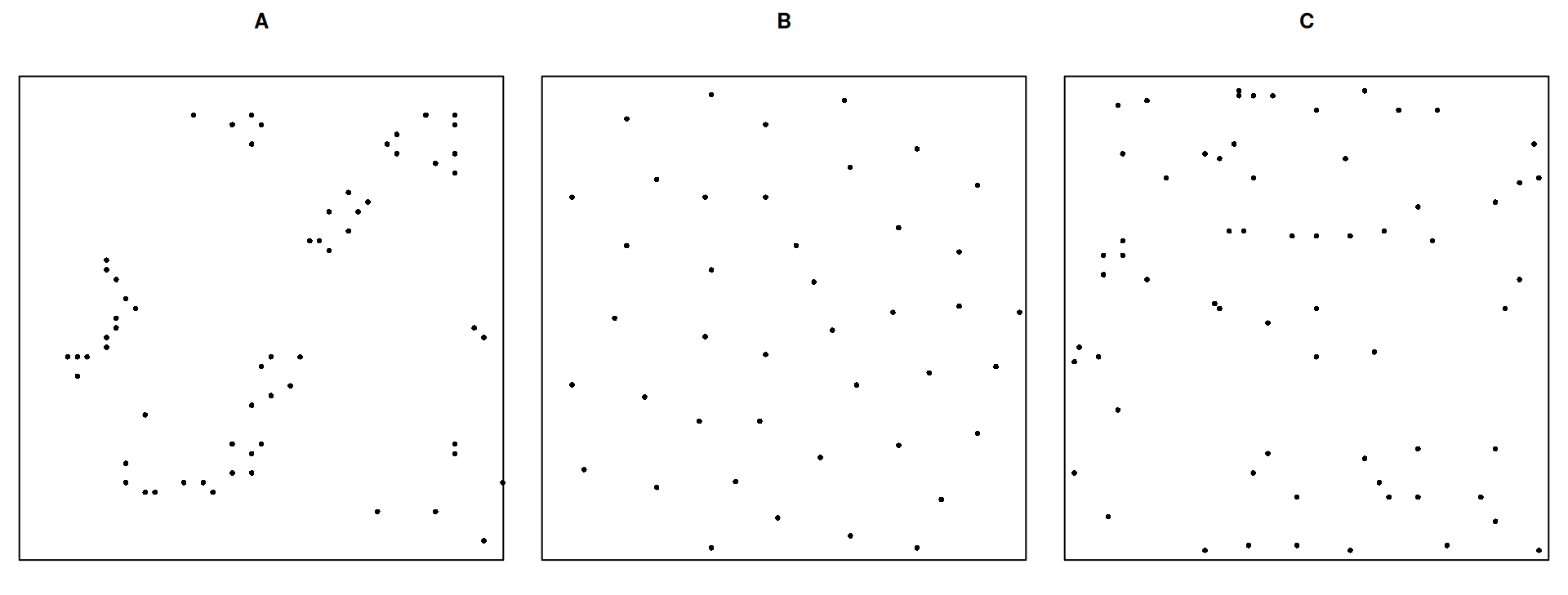
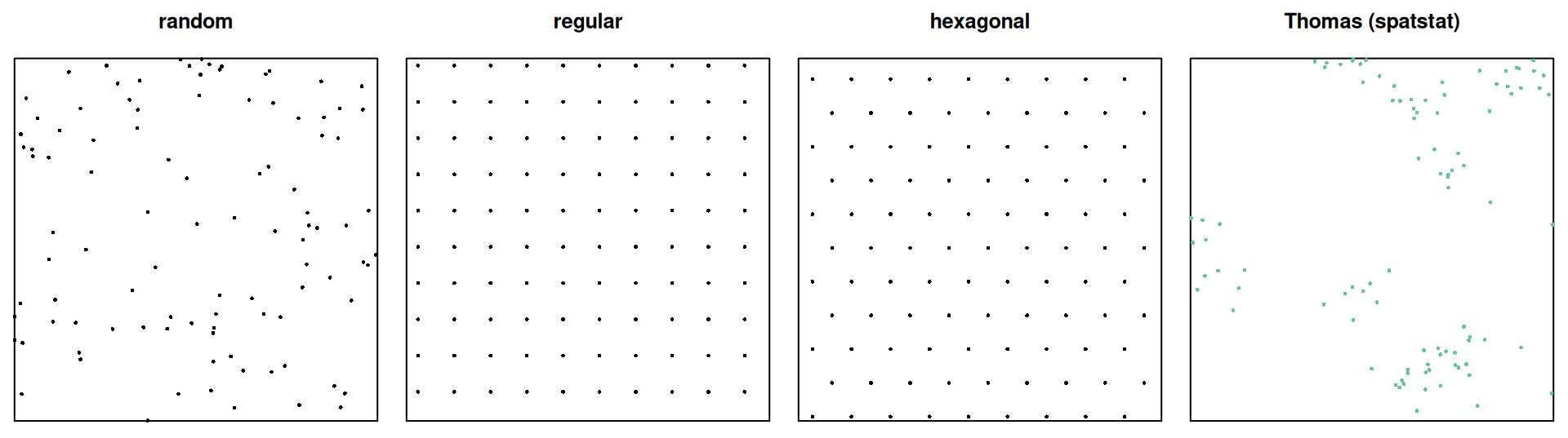
Which one is completely random?

Point processes

From process to pattern

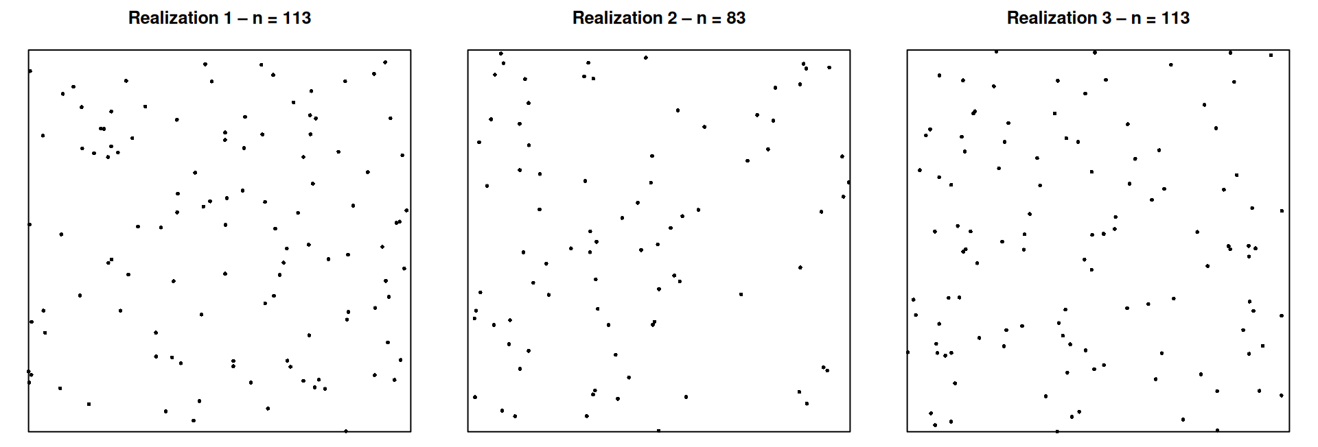
• A point process is a stochastic process whose realization is a set of points: the point pattern
• We usually observe one realization in one observation window \(W\)
• Both the locations and the number of points are random
• \(N(A)\) = number of points in region \(A\), a random variable for every region \(A\)

Complete spatial randomness (CSR)

The homogeneous Poisson process with intensity \(\lambda\):

1. \(N(A) \sim \text{Poisson}(\lambda\,|A|)\) for every region \(A\)
2. Given \(n\) points, they are independent and uniformly distributed in \(W\)

No preferred locations (first order), no interaction (second order). CSR is the null model for most tests.

First- and second-order properties

• First order: intensity \(\lambda(u)\), the expected number of points per unit area at location \(u\)
  • homogeneous: \(\lambda\) constant; inhomogeneous: \(\lambda(u)\) varies (soil, slope, population, …)
• Second order: interaction. Given the intensity, do points
  • attract each other → clustered
  • repel each other → regular (inhibition)
  • ignore each other → independent (Poisson)
• Analogy: first order ≈ mean, second order ≈ covariance

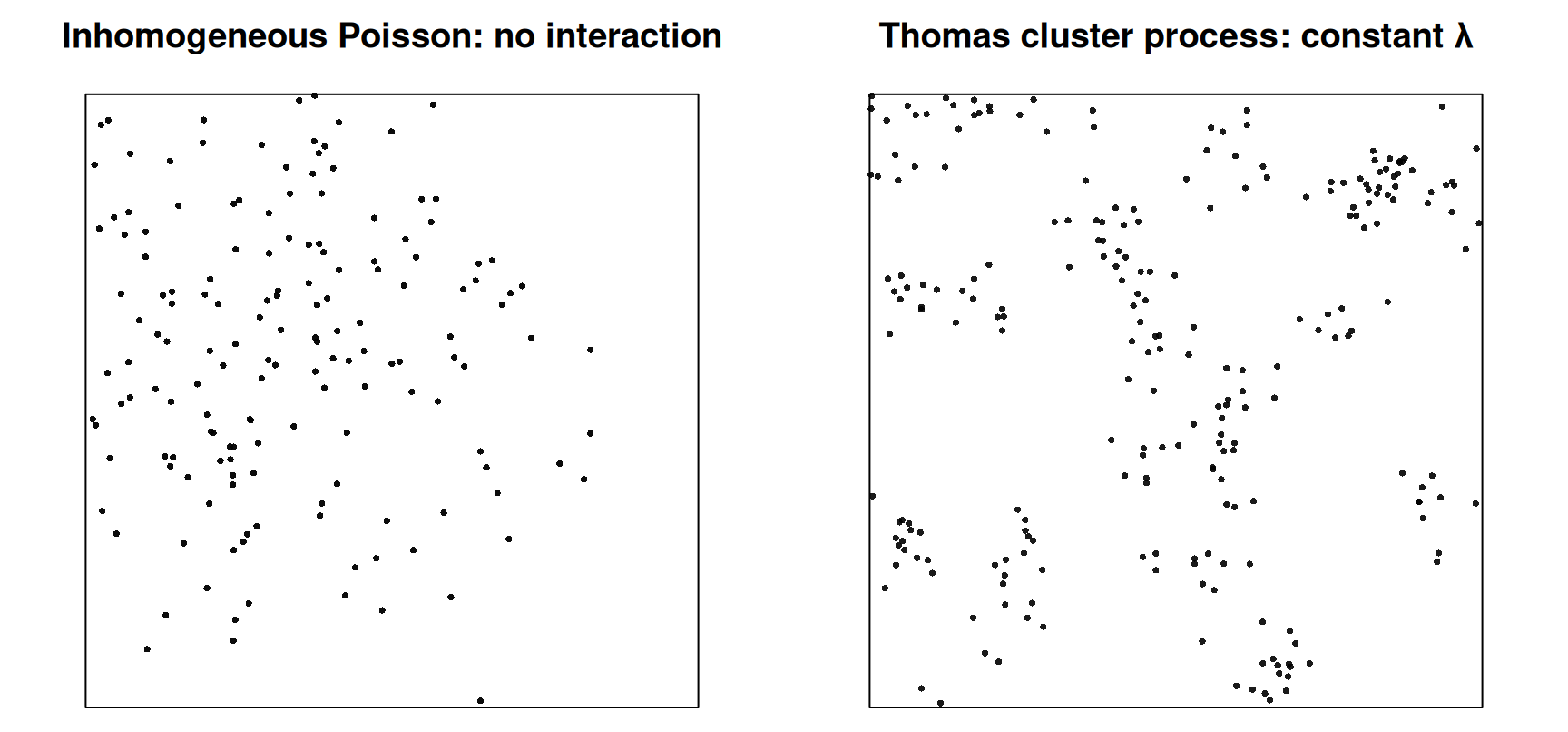
Same look, different cause

From a single pattern, these are hard to tell apart. Covariates and domain knowledge are needed.

spatstat and sf

From sf to spatstat

n <- 30
set.seed(13531)
xy <- data.frame(x = runif(n), y = runif(n)) |>
  st_as_sf(coords = c("x", "y"))
w1 <- st_bbox(c(xmin = 0, ymin = 0, xmax = 1, ymax = 1)) |> st_as_sfc()  # square
w2 <- st_sfc(st_point(c(1, 0.5))) |> st_buffer(1.2)                      # circle

pp1 <- c(w1, st_geometry(xy)) |> as.ppp()   # first geometry = window
pp2 <- c(w2, st_geometry(xy)) |> as.ppp()
pp1

Planar point pattern: 30 points
window: polygonal boundary
enclosing rectangle: [0, 1] x [0, 1] units

…and back to sf

st_as_sf(pp1) |> head(4)

Simple feature collection with 4 features and 1 field
Geometry type: GEOMETRY
Dimension:     XY
Bounding box:  xmin: 0 ymin: 0 xmax: 1 ymax: 1
CRS:           NA
   label                           geom
1 window POLYGON ((1 1, 0 1, 0 0, 1 ...
2  point    POINT (0.8878369 0.5102393)
3  point    POINT (0.6425945 0.6621732)
4  point    POINT (0.2986297 0.9070111)

The window comes back as a feature with label = "window", the points with label = "point".

Observation window

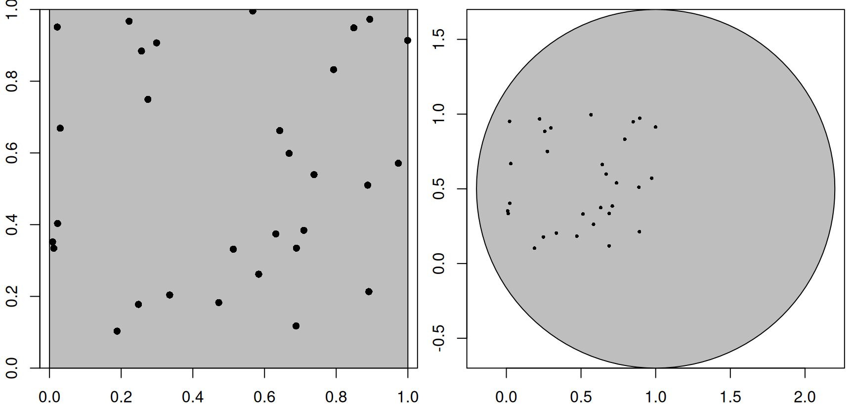
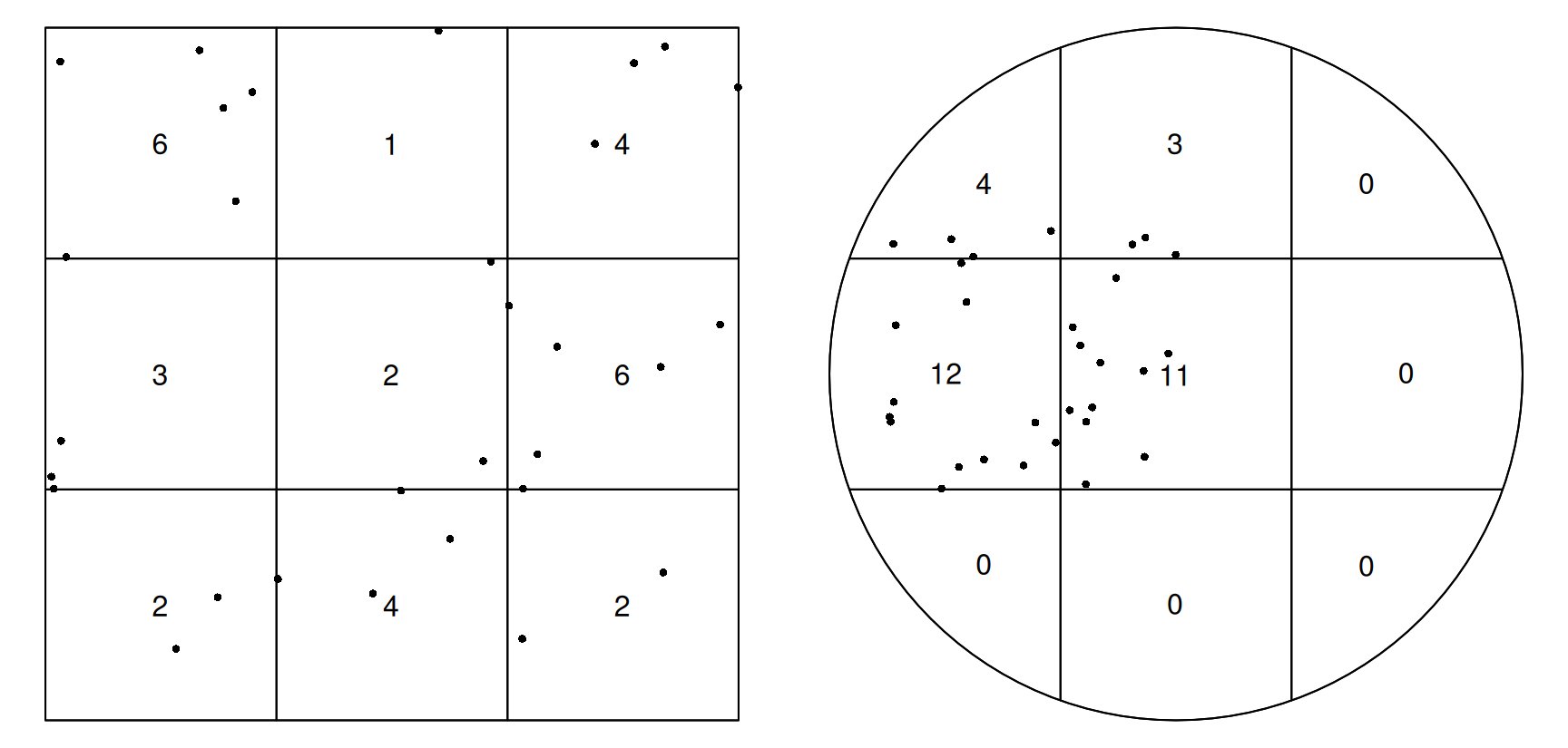
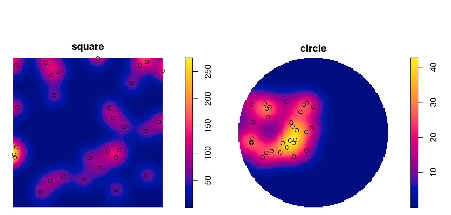
Same points, different window

   square    circle 
30.000000  6.634487 

Quadrat counts depend on the window

Density depends on the window

The window is part of the data: it defines where points could have occurred. Defaults like the bounding box or convex hull are guesses.

Coordinate reference systems

spatstat needs planar coordinates

nc  <- read_sf(system.file("gpkg/nc.gpkg", package = "sf"))
pts <- st_centroid(st_geometry(nc))      # ellipsoidal coordinates (NAD27)
try(as.ppp(pts))

Error : Only projected coordinates may be converted to spatstat class objects

nc_p <- st_transform(st_geometry(nc), "EPSG:32119")   # NC State Plane, metres
pp_nc <- c(st_union(nc_p), st_centroid(nc_p)) |> as.ppp()
pp_nc

Planar point pattern: 100 points
window: polygonal boundary
enclosing rectangle: [123829.8, 930518.6] x [14740.1, 318255.5] units

Why does it matter?

• spatstat computes Euclidean distances and areas
• On longitude/latitude, one degree of longitude shrinks from ~111 km at the equator to 0 at the poles
  • intensity (points per area) and K functions (distances) would be distorted
• Small study area: any suitable projected CRS (Münster: UTM 32N, EPSG:25832)
• Large area: no projection preserves distances and areas everywhere
  • intensity → use an equal-area projection
  • global patterns → treat them on the sphere (see §11.5, end of lecture)

First order: intensity

Example: Barro Colorado Island trees

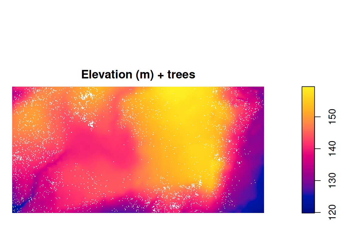
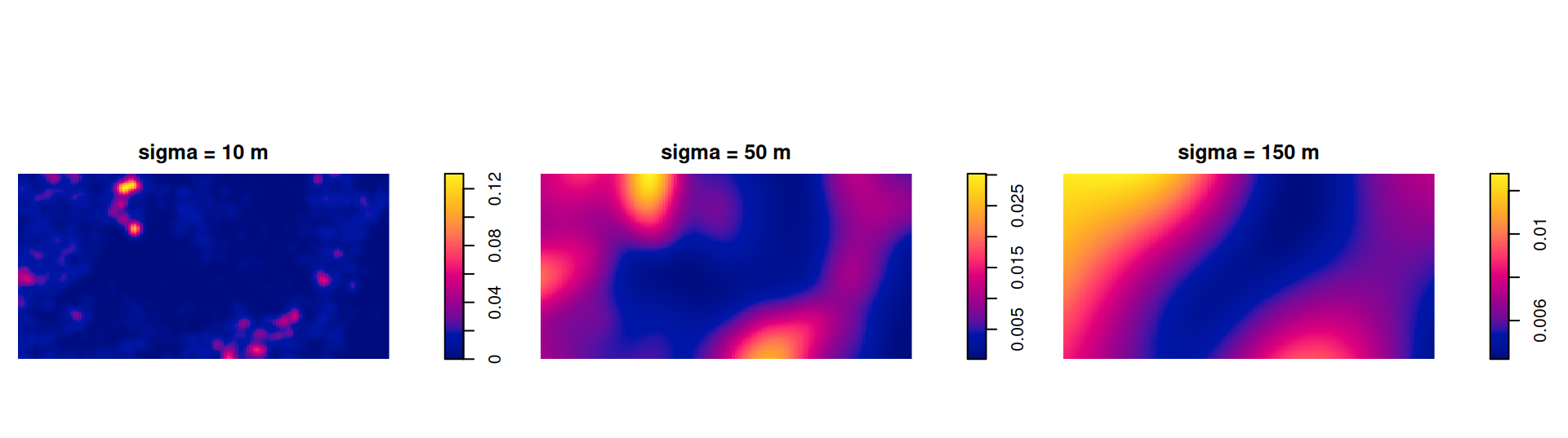
• bei: 3604 trees of Beilschmiedia pendula in a 1000 × 500 m plot (Panama)
• bei.extra: covariates elevation (elev) and slope (grad)

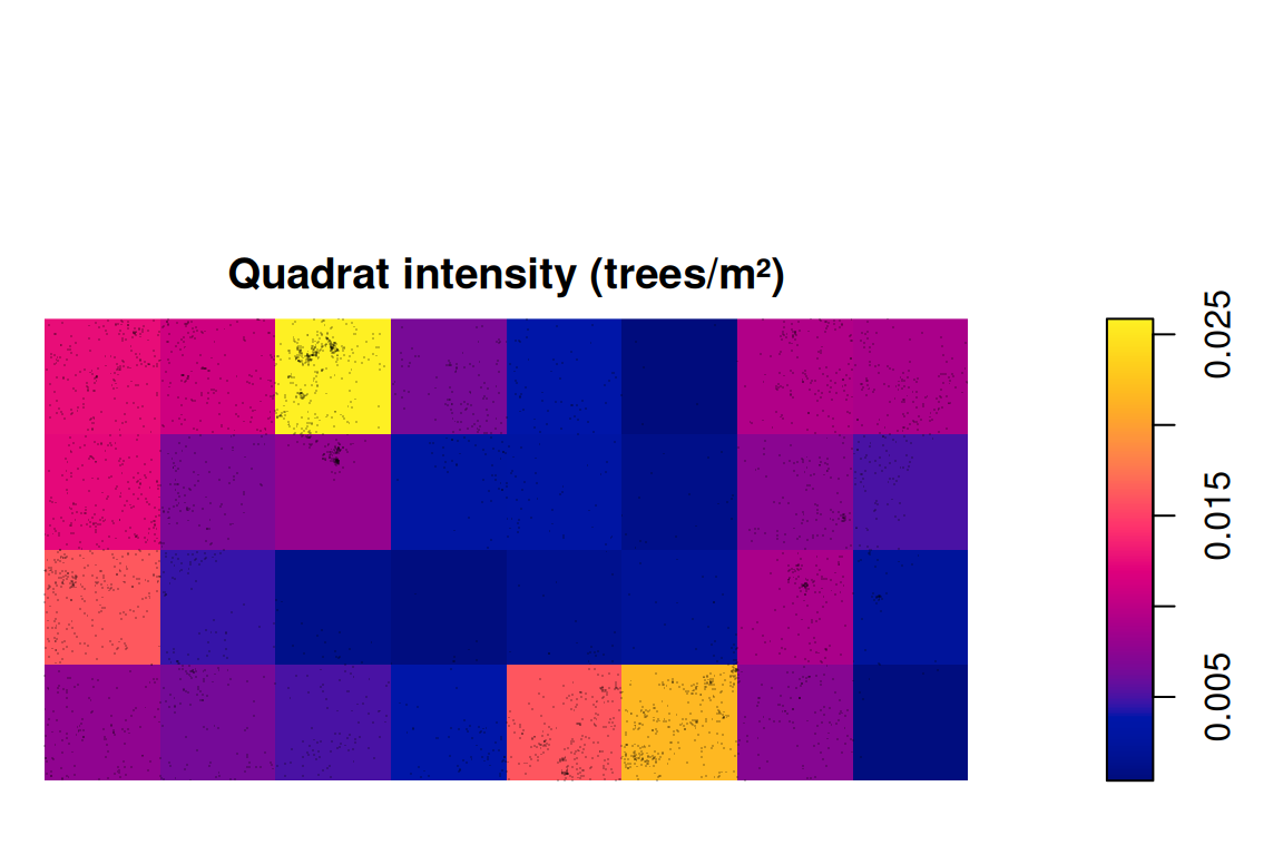
Homogeneous intensity and quadrats

[1] 0.007208

The single number \(\hat\lambda = n/|W|\) hides a lot of variation.

Kernel density: the bandwidth matters

     diggle scott.sigma 
   2.813112   56.125350 

Gaussian kernel with edge correction.

Bandwidth selectors (bw.diggle, bw.ppl, bw.scott, bw.CvL) can disagree a lot.

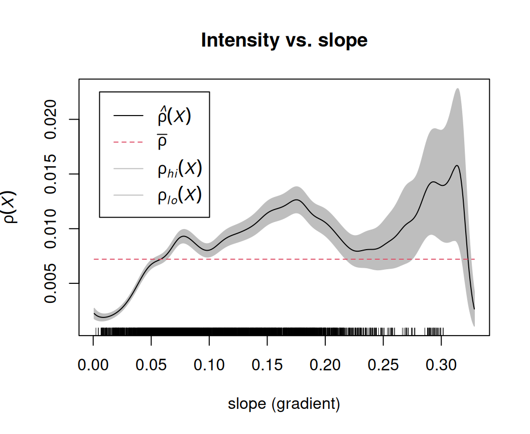
Intensity as a function of a covariate

• Non-parametric estimate of \(\lambda\) as a function of slope
• Trees prefer steeper slopes
• Next step: a parametric model with ppm() (later)

Testing CSR with quadrat counts

\[\chi^2 = \sum_{\text{quadrats}} \frac{(\text{Observed} - \text{Expected})^2}{\text{Expected}}, \qquad \text{Expected} = \frac{n}{\#\text{quadrats}}\]

    Chi-squared test of CSR using quadrat counts

data:  bei
X2 = 781.26, df = 7, p-value < 2.2e-16
alternative hypothesis: two.sided

Quadrats: 4 by 2 grid of tiles

    Conditional Monte Carlo test of CSR using quadrat counts
    Test statistic: Pearson X2 statistic

data:  pp1
X2 = 7.8, p-value = 0.892
alternative hypothesis: two.sided

Quadrats: 9 tiles (irregular windows)

Second order: interaction

Nearest-neighbour distances

Clark–Evans index: \(R = \dfrac{\bar d_{\text{observed}}}{\bar d_{\text{CSR}}}\) with \(\bar d_{\text{CSR}} = \dfrac{1}{2\sqrt{\lambda}}\)

\(R < 1\) clustered, \(R \approx 1\) random, \(R > 1\) regular

pats <- list(random = japanesepines, clustered = redwood, regular = cells)
sapply(pats, clarkevans, correction = "Donnelly")

   random clustered   regular 
1.0075072 0.5849906 1.5604256 

clarkevans.test(redwood, alternative = "clustered")

    Clark-Evans test
    Donnelly correction
    Z-test

data:  redwood
R = 0.58499, p-value = 1.906e-11
alternative hypothesis: clustered (R < 1)

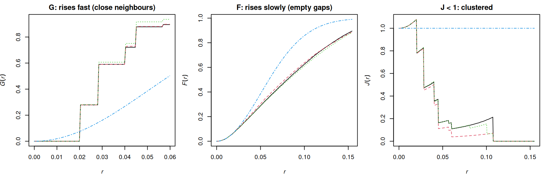
G, F and J functions

• \(G(r)\): distribution of the distance from a point to its nearest point (event to event)
• \(F(r)\): distribution of the distance from an arbitrary location to the nearest point (empty space)
• \(J(r) = \dfrac{1 - G(r)}{1 - F(r)}\): \(J = 1\) CSR, \(J < 1\) clustered, \(J > 1\) regular

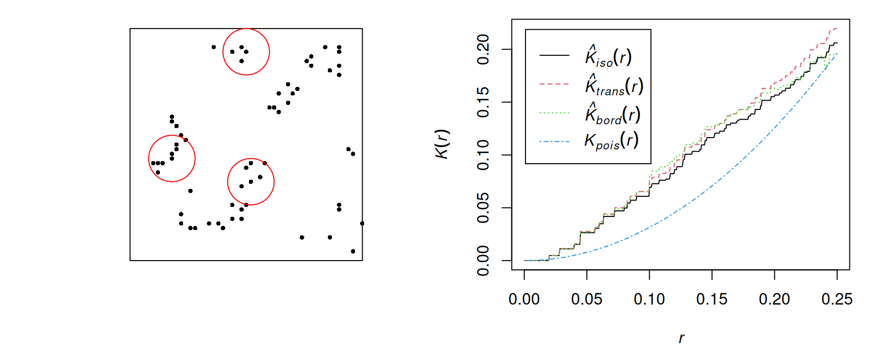
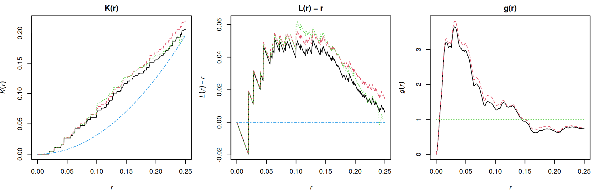
Ripley’s K function

\(\lambda K(r)\) = expected number of other points within distance \(r\) of a typical point

\[\hat K(r) = \frac{|W|}{n(n-1)} \sum_i \sum_{j \neq i} \mathbf{1}(d_{ij} \le r)\, e_{ij}, \qquad K_{\text{CSR}}(r) = \pi r^2\]

\(e_{ij}\) is the edge correction: neighbours outside \(W\) are never seen (border, translation, isotropic corrections).

L function and pair correlation

• \(L(r) = \sqrt{K(r)/\pi}\): under CSR \(L(r) = r\), so we plot \(L(r) - r\) (zero under CSR)
• \(g(r) = K'(r) / (2\pi r)\): non-cumulative, refers to pairs at distance exactly \(r\)
  • \(g > 1\): clustering at that distance; \(g < 1\): inhibition

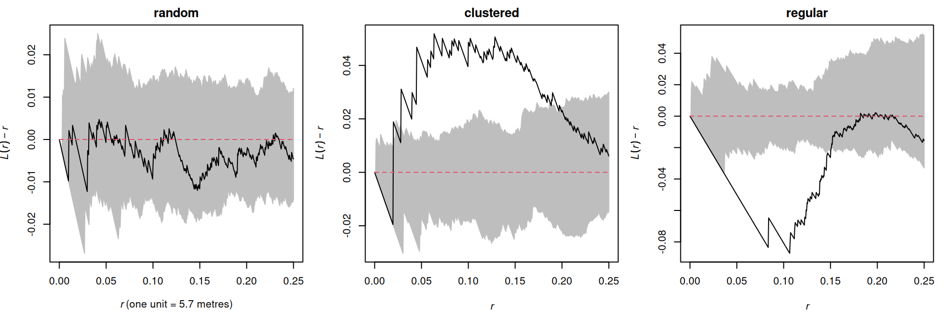
Monte Carlo envelopes

Simulate nsim CSR patterns (same \(n\), same \(W\)), compute the function for each, and take the min/max as a band.

Above the band: clustered at that distance. Below: regular.

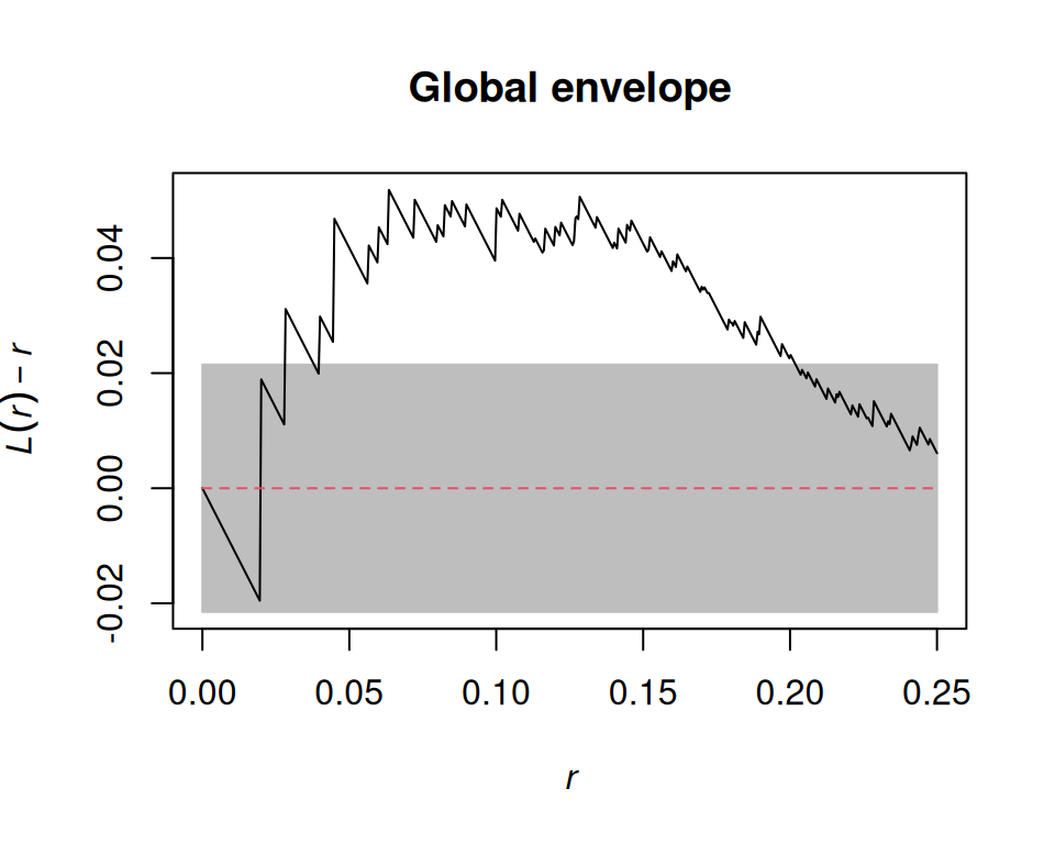
Pointwise vs. global envelopes

• Pointwise (default): with nsim = 39, the significance level of 5% holds only for one distance \(r\) chosen in advance. Scanning all \(r\) is multiple testing.
• Global (global = TRUE): a band for the whole curve at once, with α = 1/(nsim + 1)

[1] 0.01

Marked point patterns

Marks (book §11.3)

• Categorical (multitype): species, crime type, case/control
• Continuous: tree diameter, earthquake magnitude, number of victims

Simple feature collection with 3 features and 2 fields
Geometry type: GEOMETRY
Dimension:     XY
Bounding box:  xmin: 0 ymin: 0 xmax: 200 ymax: 200
CRS:           NA
   spatstat.geom..marks.x.  label                           geom
NA                      NA window POLYGON ((0 0, 200 0, 200 2...
1                     32.9  point                POINT (200 8.8)
2                     53.5  point               POINT (199.3 10)

Marked planar point pattern: 584 points
Mark variables: spatstat.geom..marks.x., label 
window: rectangle = [0, 200] x [0, 200] units

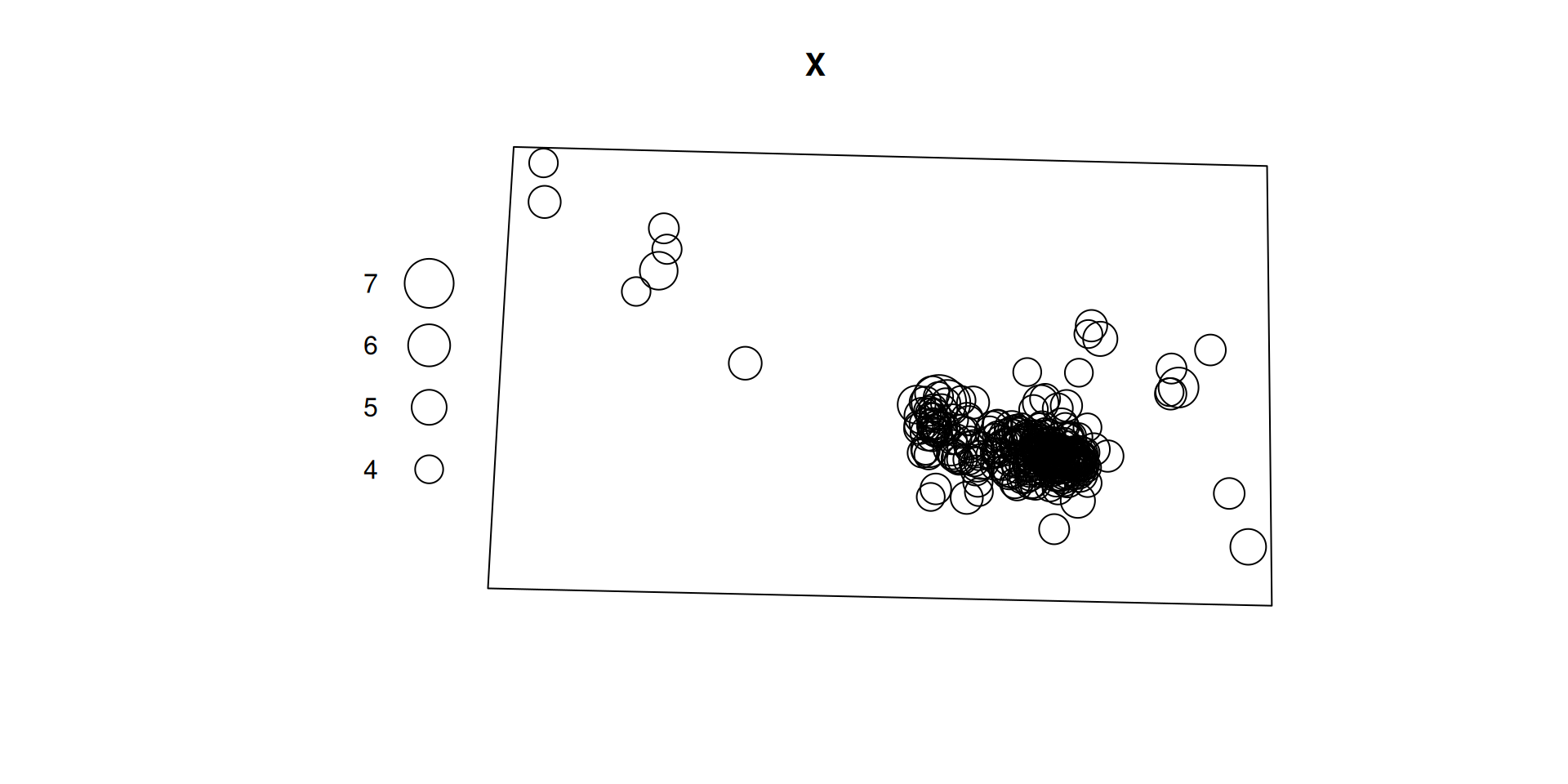
Earthquakes Nepal 2015

url <- paste0(
  "https://earthquake.usgs.gov/fdsnws/event/1/query?format=csv",
  "&starttime=2015-04-25&endtime=2015-12-31",
  "&minlatitude=26.3&maxlatitude=30.5&minlongitude=80&maxlongitude=88.3",
  "&minmagnitude=4&orderby=time-asc")
eq <- read.csv(url)

eq_sf <- st_as_sf(eq, coords = c("longitude", "latitude"), crs = 4326) |>
  st_transform(32645)                       # UTM 45N, metres

win <- st_bbox(c(xmin = 80, ymin = 26.3, xmax = 88.3, ymax = 30.5),
               crs = st_crs(4326)) |>
  st_as_sfc() |> st_segmentize(10000) |> st_transform(32645)

X <- as.ppp(st_geometry(eq_sf), W = as.owin(win))
marks(X) <- eq_sf$mag
plot(X)

Point patterns on linear networks

Why networks?

• Many events can only occur on a network: traffic accidents, street crime, street trees, ambulance calls, spines along a dendrite
• Planar methods assume points could be anywhere in \(W\)
• Euclidean distance ≠ shortest-path distance along the network
• Intensity is per unit length (accidents per metre of street), not per area

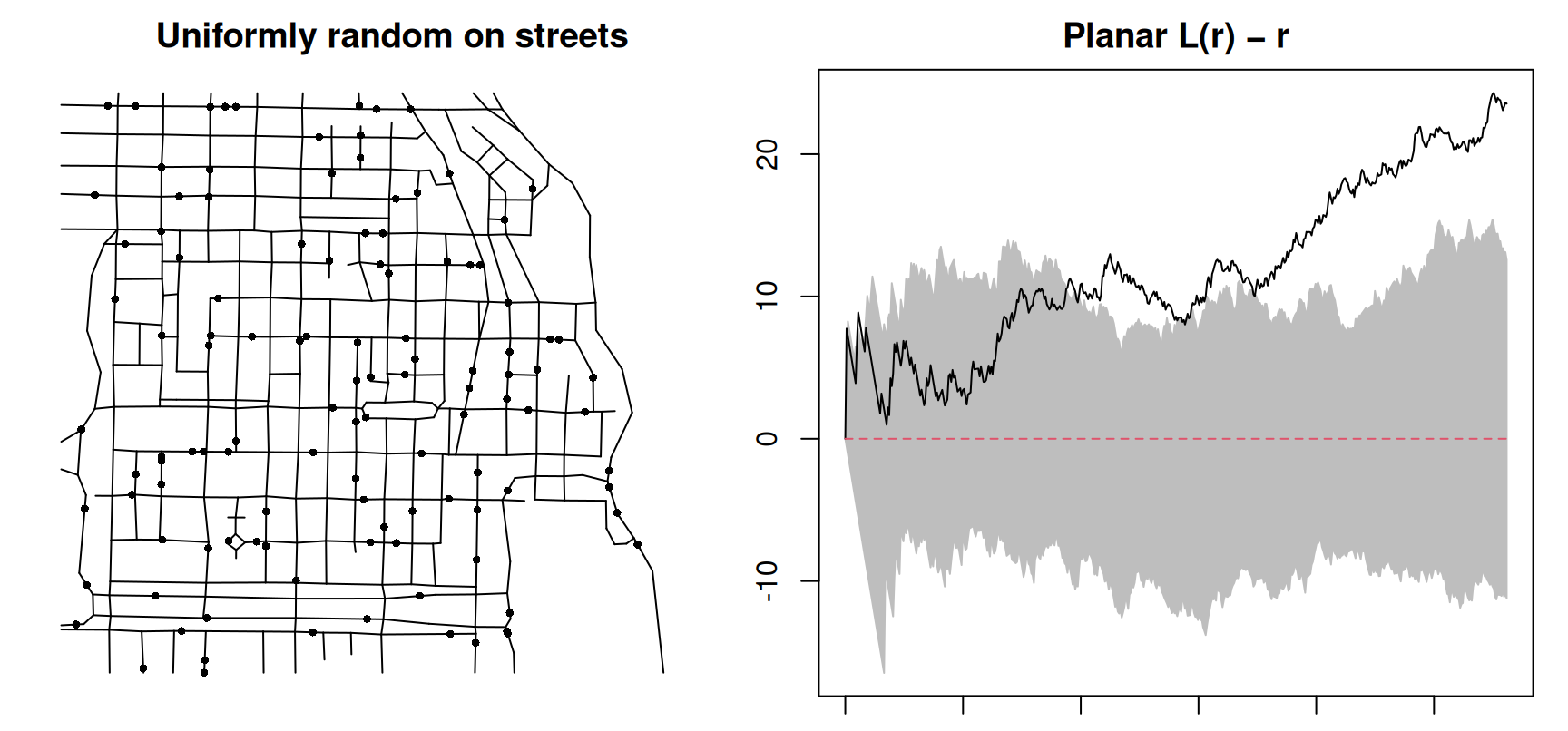
Random on streets ≠ random in the plane

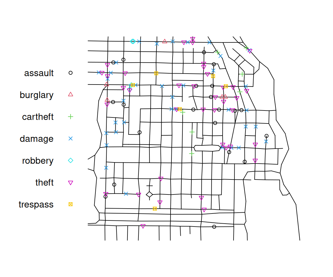
spatstat classes: linnet and lpp

Point pattern on linear network
116 points
Multitype, with possible types: 
   assault burglary cartheft damage robbery theft trespass
Linear network with 338 vertices and 503 lines
Enclosing window: rectangle = [0.3894, 1281.9863] x [153.1035, 1276.5602] feet

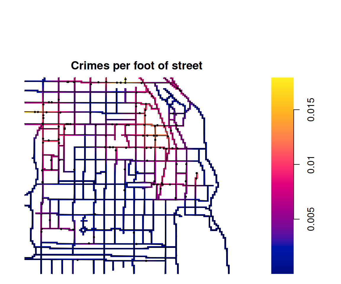
Intensity on a network

• The kernel spreads along the streets (heat equation), not across blocks
• Result is a linim: an image living on the network
• densityQuick.lpp() is a fast approximation for large networks

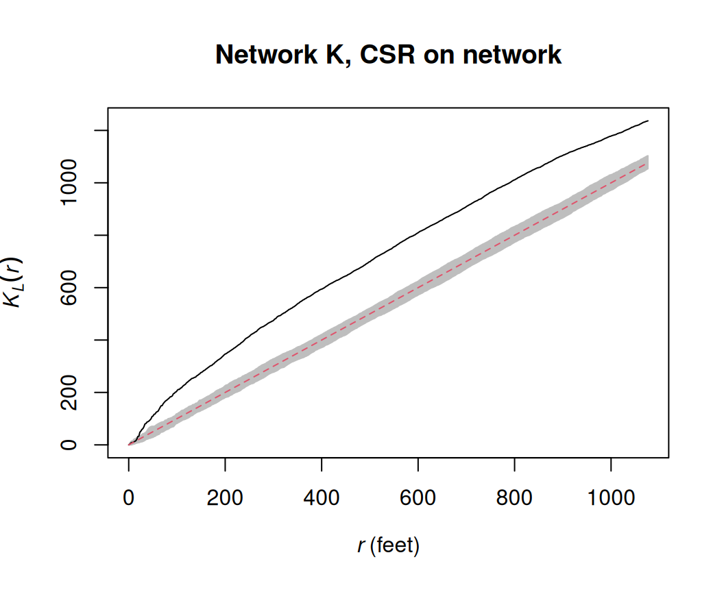
Network K function

• Distances measured along the network (shortest path)
• Normalised so that CSR on the network gives \(K_L(r) = r\)
• Here: crimes cluster even after accounting for the network

Sampling and simulation

Spatial sampling with st_sample() (book §11.4)

Any spatstat simulator can be called from sf via type =.

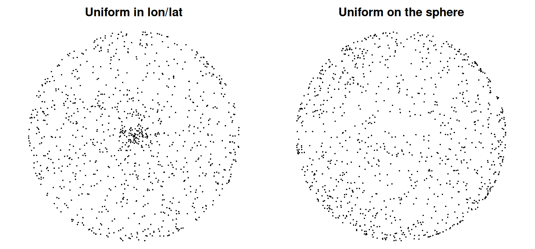
Simulating points on the sphere (book §11.5)

Uniform longitude/latitude piles points up at the poles. sf + s2 samples uniformly on the sphere.

Wrap-up

Python for your projects

• pointpats (PySAL): quadrat statistics, centrography, G/F/J/K/L functions, simulation of CSR and cluster processes
• spaghetti (PySAL): spatial networks, snapping points, network K function
• scikit-learn KernelDensity: kernel intensity estimation
• rpy2: call spatstat from Python when nothing else does the job

Summary

Question	Tools
How many, where? (first order)	intensity(), quadratcount(), density(), rhohat()
Is it random?	quadrat.test(), clarkevans.test(), envelope(global = TRUE)
Do points interact? (second order)	Gest(), Fest(), Jest(), Kest()/Lest(), pcf(); Kinhom() if λ varies
On a network?	linnet, lpp, density.lpp(), linearK(), spNetwork

References

• Pebesma, E. & Bivand, R. (2023). Spatial Data Science: With Applications in R. CRC Press. Ch. 11. https://r-spatial.org/book/
• Baddeley, A., Rubak, E. & Turner, R. (2015). Spatial Point Patterns: Methodology and Applications with R. CRC Press.
• Baddeley, A., Nair, G., Rakshit, S., McSwiggan, G. & Davies, T. M. (2021). Analysing point patterns on networks — a review. Spatial Statistics, 42, 100435.
• Gelb, J. (2021). spNetwork: A package for network kernel density estimation. The R Journal, 13(2).
• Okabe, A. & Sugihara, K. (2012). Spatial Analysis Along Networks. Wiley.